Supersymmetric gauge theory
Contents |
 SUSY in 4D (with 4 real generators)
In theoretical physics, one often analyzes theories with supersymmetry which also have internal gauge symmetries. So, it is important to come up with a supersymmetric generalization of gauge theories. In four dimensions, the minimal N=1 supersymmetry may be written using a superspace. This superspace involves four extra fermionic coordinates  , transforming as a two-component spinor and its conjugate.
Every superfield, i.e. a field that depends on all coordinates of the superspace, may be expanded with respect to the new fermionic coordinates. There exists a special kind of superfields, the so-called chiral superfields, that only depend on the variables  but not their conjugates (more precisely,
  ). However, a vector superfield depends on all coordinates. It describes a gauge field and its superpartner, namely a Weyl fermion that obeys a Dirac equation.

V is the vector superfield (prepotential) and is real ( ). The fields on the right hand side are component fields.
The gauge transformations act as
where Λ is any chiral superfield.
It's easy to check that the chiral superfield
is gauge invariant. So is its complex conjugate  .
.
A nonSUSY covariant gauge which is often used is the Wess-Zumino gauge. Here, C, χ, M and N are all set to zero. The residual gauge symmetries are gauge transformations of the traditional bosonic type.
A chiral superfield X with a charge of q transforms as


The following term is therefore gauge invariant
 is called a bridge since it "bridges" a field which transforms under Λ only with a field which transforms under
  only.
only.
More generally, if we have a real gauge group G that we wish to supersymmetrize, we first have to complexify it to Gc. e-qV then acts a compensator for the complex gauge transformations in effect absorbing them leaving only the real parts. This is what's being done in the Wess-Zumino gauge.
Differential superforms
Let's rephrase everything to look more like a conventional Yang-Mill gauge theory. We have a U(1) gauge symmetry acting upon full superspace with a 1-superform gauge connection A. In the analytic basis for the tangent space, the covariant derivative is given by  . Integrability conditions for chiral superfields with the chiral constraint
  leave us with
 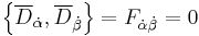 . A similar constraint for antichiral superfields leaves us with
  . This means that we can either gauge fix
  or
or  but not both simultaneously. Call the two different gauge fixing schemes I and II respectively. In gauge I,
  and in gauge II,
  . Now, the trick is to use two different gauges simultaneously; gauge I for chiral superfields and gauge II for antichiral superfields. In order to bridge between the two different gauges, we need a gauge transformation. Call it e-V (by convention). If we were using one gauge for all fields,
  would be gauge invariant. However, we need to convert gauge I to gauge II, transforming X to (e-V)qX. So, the gauge invariant quantity is
  .
.
In gauge I, we still have the residual gauge  where
where  and in gauge II, we have the residual gauge
  satisfying
  . Under the residual gauges, the bridge transforms as
 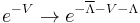 . Without any additional constraints, the bridge
  wouldn't give all the information about the gauge field. However, with the additional constraint
  , there's only one unique gauge field which is compatible with the bridge modulo gauge transformations. Now, the bridge gives exactly the same information content as the gauge field.
Theories with 8 or more SUSY generators
In theories with higher supersymmetry (and perhaps higher dimension), a vector superfield typically describes not only a gauge field and a Weyl fermion but also at least one complex scalar field.